Tree

Suppose we we are given the following tree.

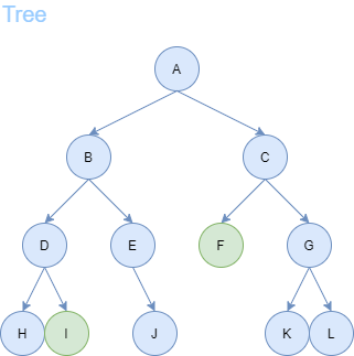
The adviser asks us to find the path from the start node A to any goal node F or I.

Breadth First Search (BFS)

We first attempt this problem with Breadth First Search. Using a Queue data structure, we expand from the starting node A until a goal node is found.

After 6 steps, we find the goal node F. From goal node F, we backtrack to the predecessors until we arrive back to the starting node A. We receive a path of length = 3.

Checkpoint: Breadth First Search expands layer by layer. This means that the path returned by BFS will always be the shortest path from the starting node to any goal node.

Depth First Search (DFS)

We attempt this search problem once again, this time using Depth First Search. Depth First Search can be implemented like BFS, however using a Stack instead of a Queue.

After 5 steps, we find the goal node I. From goal node I, we backtrack to the predecessors until we arrive back to the starting node A. We receive a path of length = 4.

DFS can also be implemented as a recursive algorithm.

function dfs(node):
    if node is a goal:
        return node

    for all children of node:
        if dfs(child) is a valid path:
            return node + path returned by child
    
    return no valid path

Checkpoint: Is the path returned by DFS always going to be the shortest path? When should we use DFS over BFS?

From Graphs to Trees

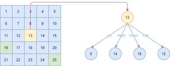
We can apply the algorithms above to all different type of graphs as long as we know the actions that the agent can take to transition from one state to the next.

Uniform Cost Search (UCS) & Dijkstra’s Algorithm

Uniform Cost Search is a generalization of BFS that works on weighted graphs. It behaves in a similar manner with Dijkstra’s Algorithm. The major (if not only) difference is: unlike Dijkstra’s Algorithm, Uniform Cost Search terminates when the first goal node is found.

Suppose we wish to find the shortest path from starting node A to goal node C.

Define g(n) as the actual cost from reaching node n from the initial node. Using a Min Priority Queue, we expand based on order of minimum g(n).

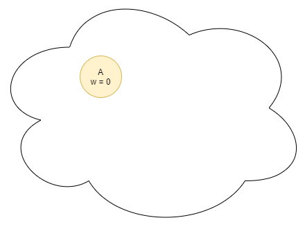
Begin the algorithm with the Priority Queue containing only the starting node A with priority = g(n) = 0.

Iterate while the Priority Queue is not empty. Pop the current head off, clear the node, and add it’s non-cleared children to the Priority Queue with weight g(child).

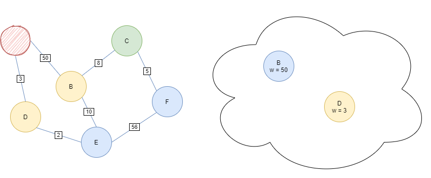
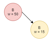
If the child already exists inside the queue, update it’s value if the new priority is smaller than the original.

UCS is complete when a goal node has been found or the queue is empty; no valid path exists. The whole process should look something like this:

Heuristic Functions

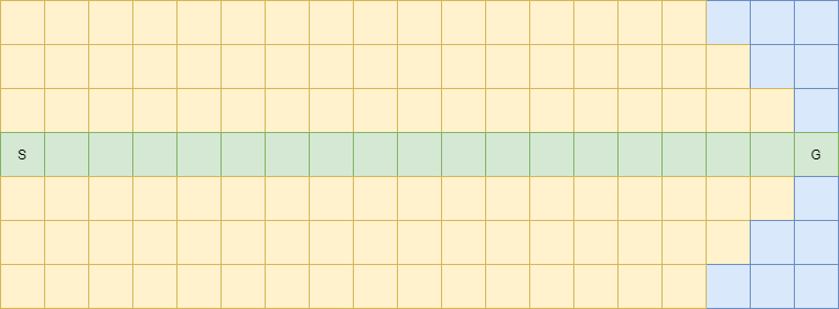
While BFS and UCS are algorithms that can find the shortest path, it’s running time is not so great on bigger graphs. Suppose were asked to find the shortest path in the graph below:

By the time BFS or UCS finishes, almost the entireity of the graph have been expanded.

We wish to reduce the computational power needed to find such a path. We do this by defining two additional functions:

h(n) - an estimated cost of reaching any goal node from node n

f(n) - g(n) + h(n) - the heuristic cost, an estimated tally of how close any node n is to any goal node

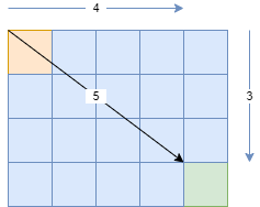
In a Cartesian graph where the edges all have the same weight, the heuristic function h(n) is typically implemented as the Manhattan distance or the Euclidean distance.

h1(n): Manhattan distance = 3 + 4 = 7

h2(n): Euclidean distance = sqrt(3*3 + 4*4) = 5

Warning: h1(n) and h2(n) will likely not be great on a graph where edges take on multiple possible weights (if calculating h1(n) and h2(n) is possible at all). A different estimated cost function will most likely be necessary.

Heuristic (A*) Search

A* improves upon BFS and UCS by expanding in order of minimum f(n), the heuristic cost. Therefore, implementing A* should require a very simple modification the existing UCS procedure.

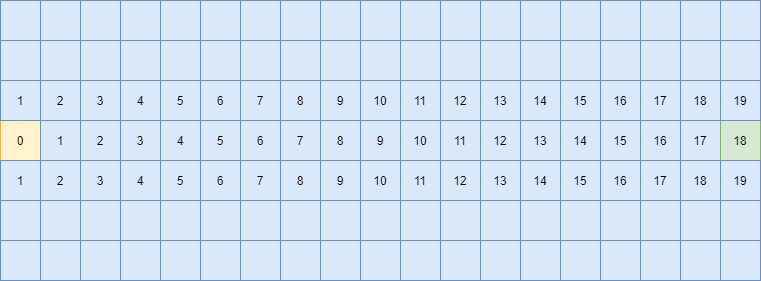
Let’s expand the graph above. We begin by assuming that each edge has a weight of 1. Then, each relevant node has g(n) cost as follows:

Furthermore, each relevant node has an estimated cost h1(n) as follows:

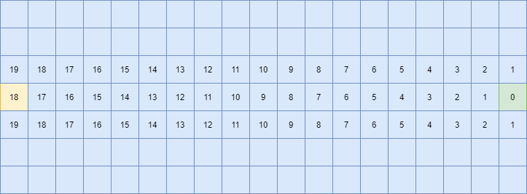
We expand our graph based on f(n) using h1(n). Our graph will be expanded as follows:

It is evident that the amount of nodes expanded is significantly smaller than the expansion provided by both BFS and UCS.